Deseq2 Analysis Basics
We’re going to use an R package called DESeq2. It has extensive documention here:
The vignette is particularly useful, and is frequently updated. You’ll be learning a small subset of it today, which should give you a foundation to explore the extent of DESeq2’s functionality.
The basic steps in abstract
Before we get into the actual code we’ll be using, here’s a quick outline of the analysis:
- Load DESeq2 R library
- Read in Count Data
- Read in Experiment Design
- Combine Data & Design into DDS object
- Run DESeq
- Data Interpretation - the hard part
A lot of the work above is in loading the data into R, and then making sure they are formatted correctly. Once this is done, running DESeq is fairly straightforward.
The two main pieces of data we need for steps 2 and 3:
- a table of the counts
- the experiment design
First, let’s clean up our directory a bit:
$ ls
shows:
dm_counts_s2.txt                      SRR5457510_1.bam
dm_counts_s2.txt.summary              SRR5457511_1.bam
dm_fcounts.slurm.sh                   SRR5457512_1.bam
dm_fcounts.slurm.sh~                  SRR5457513_1.bam
feature_counts.dm_run01.57865896.err  SRR5457514_1.bam
feature_counts.dm_run01.57865896.out  SRR5457515_1.bam
We’ll move the bam files into their own directory, and then create a directory to do our DESeq analysis.
$ mkdir bams
$ mv *bam bams/
$ mkdir deseq
$ mv dm_counts_s2.txt deseq/
$ ls
bams   dm_counts_s2.txt.summary  feature_counts.dm_run01.57865896.err
deseq  dm_fcounts.slurm.sh       feature_counts.dm_run01.57865896.out
We also moved the counts into the deseq folder.
Let’s copy an experimental design file in the /proj/seq/data/carpentry/deseq_dm/ directory, which also has an R analysis script.
$ cd deseq/
$ cp /proj/seq/data/carpentry/deseq_dm/dm_sampleInfo.txt .
$ cp /proj/seq/data/carpentry/deseq_dm/deseq2.project_dm.R .
$ ls
Now, let’s look at the experimental design file we’ll be using. The design is a list of all the samples and what experimental conditions are assigned to them - at a minimum control vs treated.
$ less dm_sampleInfo.txt
Which shows:
sample,condition
SRR5457510,3LW
SRR5457511,3LW
SRR5457512,24hAPF
SRR5457513,24hAPF
SRR5457514,44hAPF
SRR5457515,44hAPF
We have the name of each sample in the first column labelled sample and a single experimental condition condition. In this case, samples are different stages of fly wing development. You could have more than one condition, addition comma separated columns can be added. The column names can be anything you want, but keeping them relatively simple will make things easier.
If your counting run didn’t work, you can copy the counts file from my scratch space:
cp /work/users/t/r/tristand/project_dm/deseq/dm_counts_s2.txt .
So we should have the following files:
$ ls -1
deseq2.project_dm.R
dm_counts_s2.txt
dm_sampleInfo.txt
Now we’re all set to use DESeq2 to analyze the data.
R
R is a powerful, and free, statistics package. Many things are possible with R, and we’re only going to scratch the surface.
The above is a great resource, available both online for free and in print form. Its a general introduction, so its not specifically geared toward bioinformatics analyses, but the basic principles hold.
Running R on Longleaf
As with other programs, we need to load the R module:
$ module load r
$ module list
Currently Loaded Modules:
  1) r/4.1.3
The main thing to note here is the module is lowercase r while the command to invoke is uppercase R
We’re going to run R interactively, so we’re going to use a different slurm command - srun
$ srun -p interact --pty R
We’re asking for the interactive queue with -p interact and --pty actually indicates to run in interactive mode. In theory we could let this run on the general queue, but the nodes in interact are specifically reserved for interactive jobs.
One of the things you’ll notice is our prompt is now > instead of $ - this is just the prompt style of R.
We’re no longer working in the shell, so the commands you learned don’t apply anymore. Instead we’re using R commands. technically there is a way, but we won’t go into that
Step 1: load DESeq2 library
Similar to the modules system, R doesn’t have all its packages loaded at once. An important difference is that adding R packages is adding function code (and thus memory usage) to the R instance. In addition, many packages might use the name for functions which do wildly different things.
> library("DESeq2")
This looks fairly simple, partly because ITS Research Computing has already added many packages. If you install R on your own laptop, you’ll have to install the packages yourself. See section at the end.
Formatting data
Deseq wants data in a particular format, there are several ways to get to this format depending on how you generated it in the first place. The steps we will follow are for the table format we produced with featureCounts
Step 2: read in count data
> Counts_bbmap <- read.table("dm_counts_s2.txt", header = TRUE, row.names=1)
read is a function that reads from a file, and we are specifying to read in a table format.
header = True means to read the first line as column headers
row.names=1 means the first column contains names for each row
The <- is the assignment operator in R, it is like the = in the shell. We’re assigning the data returned by read.table to the variable Counts_bbmap
The counts are getting written into a data frame, a data structure in R that allows easy access to specific columns and rows
R has a head function much like the Unix shell we can use to get a quick idea of what the data looks like
> head(Counts_bbmap)
After each of the formatting steps below, we’ll use head to see what changes have occurred.
Step 2a: remove unneeded columns
> CountTable <- Counts_bbmap[,6:11]
Most of the columns created by featureCounts are unneeded by DESeq, so we’re going to remove them.
[,6:11] this syntax means we’re taking all the rows (nothing before the comma) and only columns 6 through 11 - we have 6 data rows.
Note, we’ve assigned this cropping of the data to a new variable:
> head(CountTable)
Step 2b: truncate count headers to match experiment design names
> colnames(CountTable) <- sapply(colnames(CountTable), substr, 0,10)
featureCounts names each column of the counts by the name of the file, but in our experiment design file, we just use the names of the sames. Eg sample SRR5457511 in the design file corresponds to SRR5457511_1.bam in the counts file, so we need to remove the .bam, or in this as, we’re using the substr function to just keep the first 10 characters of the column name.
What’s happening here is colnames is fetching all the column names in CountTable, sapply is applying the substr function to each of these names. Then, we take that list and put it back into the data structure using colnames again.
> head(CountTable)
Step 3: read in experiment design
> sampleInfo <- read.csv("dm_sampleInfo.txt")
Here, we use read’s method for csv (Comma Separated Values) files.
> head(sampleInfo)
Step 3a: format for DDS object
> sampleInfo <- DataFrame(sampleInfo)
Here, we convert sampleInfo into a data frame from a simple matrix.
> head(sampleInfo)
Data frames are an special R data type that basically store a table of data, with identifiers for the rows and columns.
Step 4: Make DDS object
> dds <- DESeqDataSetFromMatrix(countData = CountTable, colData = sampleInfo, design = ~condition)
By default, R chooses the reference level alphabetically. Thus, if you had a condition ‘genotype’ with levels ‘wildtype’ and ‘mutant’, ‘m’ comes before ‘w’ in the alphabet, so ‘mutant’ will be considered the reference level. There are a number of ways to change this, two of which are:
note these first two are just examples and won’t work with the current data set
> dds$condition <- factor(dds$condition, levels = c("wildtype","mutant"))
or
> dds$condition <- relevel(dds$condition, ref = "wildtype")
This has to be done before the next step. So, for our data, do the following, which sets the earliest time point as the reference level:
> dds$condition <- relevel(dds$condition, ref = "3LW")
Step 5: Run Deseq2 analysis
> dds <- DESeq(dds)
This is it, the big analysis step! Exciting, right?
Or just anti-climatic, as I said earlier, most of the work is in getting the data formatted correctly, DESeq running is fairly straightforward.
Convert results into more useable format
> res <- results(dds)
We can look at the data:
> res
But what does all this mean? We can use mcols to get some details that the results data structure provides:
> mcols(res, use.names=TRUE)
or
> mcols(res)$description
[1] "mean of normalized counts for all samples"
[2] "log2 fold change (MLE): condition 44hAPF vs 3LW"
[3] "standard error: condition 44hAPF vs 3LW"
[4] "Wald statistic: condition 44hAPF vs 3LW"
[5] "Wald test p-value: condition 44hAPF vs 3LW"
[6] "BH adjusted p-values"
The Benjamini–Hochberg (BH) procedure is used to find adjusted p-values
We can also use the summary function:
> summary(res)
out of 12707 with nonzero total read count
adjusted p-value < 0.1
LFC > 0 (up)       : 3309, 26%
LFC < 0 (down)     : 2466, 19%
outliers [1]       : 0, 0%
low counts [2]     : 3149, 25%
(mean count < 2)
[1] see 'cooksCutoff' argument of ?results
[2] see 'independentFiltering' argument of ?results
The res function also allows for changing the p-adj value used for filtering:
> summary(res, alpha=0.05)
This only changes the numbers reported up or down:
adjusted p-value < 0.05
LFC > 0 (up)       : 3004, 24%
LFC < 0 (down)     : 2209, 17%
For the initial analysis, we set 3LW as the reference condition, but the other possible comparisons are also part of DESeq2’s algorithm. We can get results from those other possible combinations of reference vs ‘treated’ conditions without re-running the main analysis step:
> res_44hAPF_v_24hAPF <- results(dds, contrast=c("condition","44hAPF","24hAPF"))
> summary(res_44hAPF_v_24hAPF, alpha=0.05)
Here, we are just naming the new results object with description of the conditions used - again, you can come up with your own naming scheme.
Writing results to a file
> write.table(res, "dm_result_table.txt", col.names=NA, sep="\t")
This function will write the data in res to a file in the current directory (ie the one you started R in) dm_result_table.txt and will separate the columns with tabs. This table delimited text file can be read by Excel, however, note it may be quite large since we are writing results for every gene.
Filtering of data
We can use various R features make some subsets of the data, which are smaller and more convenient to work with.
Cutoff by present
> resPresent <- res[which(res$baseMean > 0),]
Here, we’re using two features of R
$ is used to indicate column identifiers within a data frame.
Thus res$baseMean accesses all the values in the baseMean column
which is a function that selects items based on a test, in this case <value> > 0 - all values greater than 0, which will trim out all except the 12707 with nonzero counts.
The results of the above are used as row selectors, so every row whose baseMean value is greater than one is selected, and are assigned to a new data frame.
Cutoff by multiple testing adjusted p-value
> resPvalCutoff <-resPresent[which(resPresent$padj<0.05),]
Here, we apply a second filtering step, this time using the padj column’s values
Order by padj
> resOrdered <- resPvalCutoff[order(resPvalCutoff$padj),]
We can also sort the data. We pull out the padj values and feed them to the order function, which returns then from lowest to highest. Because they are reordered, when we use the padj values as row identifiers, the rows are written into our new data frame in that order.
Write out the ordered Pval Cutoff results
Once we’ve done the filtering we like, we can also write out the results:
> write.table(resOrdered, "padj_005_result_table.txt", col.names=NA, sep="\t")
Checking the results with PCA
There are a variety of ways to graph and explore the data. Most of this is best done locally, for example running RStudio. The DESeq documentation linked above goes indepth into graphing.
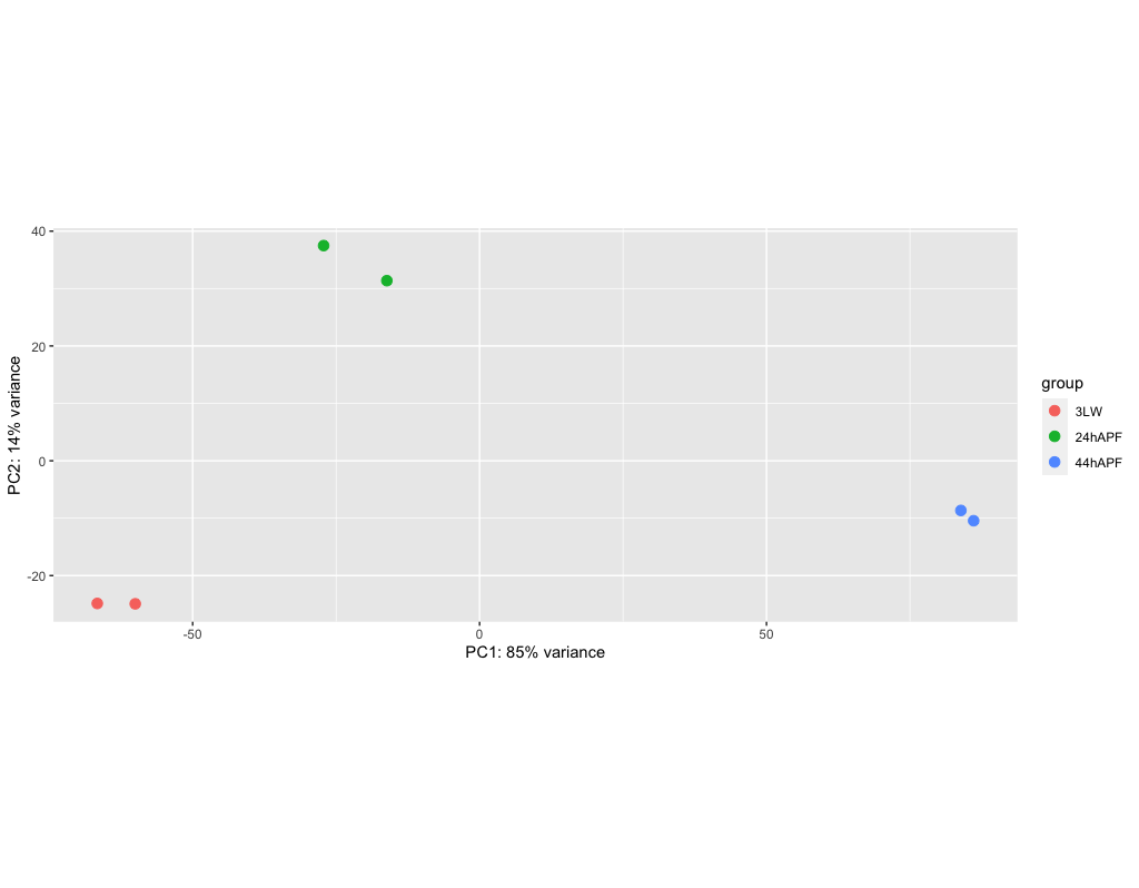
We’re going to take a look at a PCA plot of the dispersion of the data. This isn’t quite the results, but represents one of the steps taken during the analysis. However, it can give us an idea of how well the data separates out.
PCA - Principle Component Analysis - this is a method of reducing high dimensionality data by finding a rotation, or set of axes, that captures the greatest set of differences within the data.
> rld <- rlog(dds, blind=FALSE)
> png('dm_pca_rld.png')
> plotPCA(rld, intgroup=c("condition"))
> dev.off()
rlog - ‘Regularized Log’ transforms the data to Log2 scale
plotPCA - does the PCA plotting
The png and dev.off() functions are only being used to store the plot into a png file. This is a bit hack-y, but a way to make graphs and write them to a file when using a simple terminal connection. Thus, for more serious plotting, and re-plotting, of data, its best to do this locally.
We can transfer the resulting file, dm_pca_rld.png to a local machine and view the results.
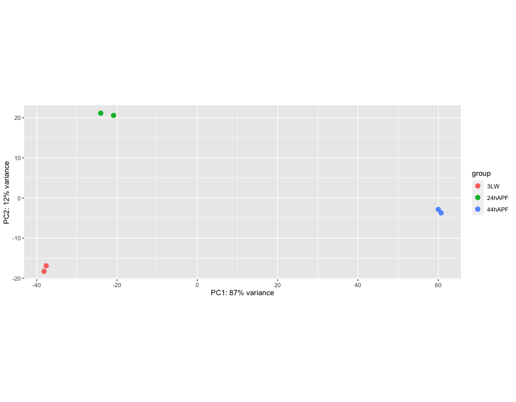
(if there is time)
This is another tranformation for PCA, it is less computationally intensive for larger date sets
> vsd <- vst(dds, blind=FALSE)
> png('dm_pca_vsd.png')
> plotPCA(vsd, intgroup=c("condition"))
> dev.off()
Quiting R and saving the session
Everything in R is a function, so quitting is also a function:
> q()
Save workspace image? [y/n/c]:
Answer ‘y’
If we look in the directory
$ ls -la
We’ll see amongs the files:
-rw-r--r-- 1 tristand its_employee_psx 12843105 Mar  7 13:18 .RData
-rw------- 1 tristand its_employee_psx      736 Mar  7 13:18 .Rhistory
R will use these to restart a session. You can download these two files and open them locally in RStudio.
Thus, you could do all the heavy lifting of running the analysis on the cluster (even submitting for example as a script), and then do all your graphing and data exploration locally.
Local installs
Note, we’re not going to do any of this section - this is FYI for running R on your own computer
We won’t go much into installing R and the very useful RStudio on a MacOS or Windows computer. You’ll have to follow the system specific instructions for your computer.
Once running R locally:
> install.packages("BiocManager")
This installs the BiocManager package which manages other packages. A lot of biostats and bioinformatics packages make use of it to make installing them easier. Once this finishes - you may need to agree to some new packages being installed, you can install DESeq2
> BiocManager::install("DESeq2", version = "3.8")
The above syntax tells R to use BiocManager’s version of installing, and it queries its own repository for DESeq2.
You may also want to install the useful ggplot2 package, which provides a lot of useful graphing capabilities.
> install.packages("ggplot2")