Differential Expression Analysis
Motivation
The basic idea behind differential expression analysis is that sequencing of RNA fragments serves as a rough proxy for how much those genes are expressed. Typically we have two or more conditions, between which we would like to know which genes have significantly changed expression levels.
Two Parts
There are two main steps in DE analyses once data is aligned.
- Quantifying counts, usually by gene
- Performing the statistical analyses on the counts between different conditions.
In this lesson, we’ll go over a bit of the theory of DE analysis and how to get the counts. In the next lesson we’ll go over a basic analysis of those counts.
Aligned data
As we touched upon in the previous lesson, alignment for DE can be to a whole reference sequence or just transcriptome
- Transcriptome alignment
- Faster – smaller target reference
- Implicit filter of non-transcribed reads, if you trust your reference transcriptome
- may not be as good with isoforms
- Whole genome alignment
- Discover new transcripts not in transcriptome annotation
- Extra time to align to larger reference less of a factor nowadays
Getting some aligned data
First, let’s get some data to work on. I’ve prepared a directory project_dm with some pre-aligned data. The data is a bit big, so we’ll want to work in our scratch space in /work/users/…
Once you cd there:
$ cp -r /proj/seq/data/carpentry/project_dm/ .
How many Biological replicates
The more biological replicates you can manage, the more robust your analysis results will be.
A little historical perspective, the MODEncode project, which wrapped up data submissions ~2011-12 required 2 biological replicates. Soon after 3 biological replicates became the recommendation, then 4.
In this paper, 48 biologial replicates were sequenced both from WT yeast and a known mutant strain. 42 of each where used to perform a variety of analyses. Unsurprisingly, the more replicates used, the more of the “full set” of changes were captured (here defined by using all the replicates).
The authors’ take away was that at least 6 biological replicates be used, preferably 12. However, practically speaking experiments cost money, and so does each additional library prepped for sequencing.
Block Design
This is also a consideration for before sequencing, when collecting the RNA experiments. In short, you want to insure you aren’t introducing artificial biases. For example, if both you and another person in the lab are sharing the work to grow/prepare/harvest your sample tissues or cell, the different experiment conditions should be divided between the individuals contributing. Similarly, if multiple batches need to be made on different days, don’t do all of the controls in one batch and all the treated/changed condition in a different batch.
Which analysis software should you use
Like other areas of bioinfomatics, there is a large number of tools that have be written.
There are many papers out there comparing many of the tools (Schurch above also includes an more recent comparison of major tools). Take a look at this Venn diagram of a comparison of three tools:
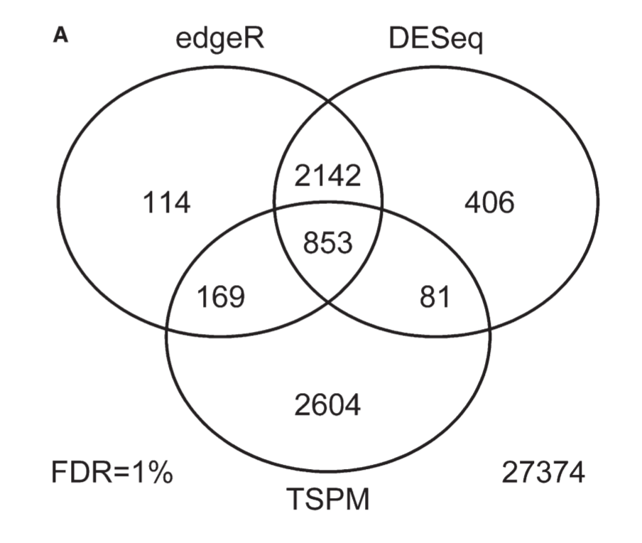
This is an older analysis, but the figure shows how all the tools agree on a subset of the data and differ on other parts.
In the previous lesson, I mentioned how the differences between aligners tend to occur with edge case read alignments, but generally agree about reads that have a single highly likely alignment. Similarly, DE tools tend to agree on genes that have the largest changes, and disagree on whether smaller expression level changes are significant.
The Shurch et al paper recommends the use of DESeq2 or edgeR when you have only 3 biological replicates.
Annotation files
When you align data, we’re only matching each read to a location on the genome. The reference genome and the alignment files, SAM or BAM, know nothing about where exons, protein binding sites, or other features exist in the genome.
This sort of meta-data is generally found in GFF or GTF files, which are tab delimited files that contain information on features in a genome, their chromosome, start and stop locations, and other information.
For all the genomes we provide in /proj/seq/data/ there are corresponding annotation files.
$ cd /proj/seq/data/
Let’s look in the dm6_UCSC directory:
$ cd dm6_UCSC
$ ls
Annotation               Drosophila_melanogaster_UCSC_dm6.tar  README.txt
Drosophila_melanogaster  NOTE                                  Sequence
Recall the index files we use to align are in the Sequence directory. The GTF files are in Annotation and its subdirectories, and for today’s lesson we’ll just be using the Genes annotations.
$ cd Annotation
$ ls
$ cd Genes
$ ls
For today’s lesson, we’ll be using genes.gtf, a detailed explanation of GTF files is here:
Briefly, it takes the following form, tab delimited fields:
<seqname> <source> <feature> <start> <end> <score> <strand> <frame> [attributes] [comments]
Let’s take a look at the one we’ll be using.
$ less -S genes.gtf
The -S is a useful option for less when viewing structured files, it disables line wrapping allowing us to view the data columns in the GTF file more clearly.
Just as a reminder, let’s see where we are:
$ pwd
/proj/seq/data/dm6_UCSC/Annotation/Genes
And the full path to the GTF is:
/proj/seq/data/dm6_UCSC/Annotation/Genes/genes.gtf
We’ll see this path in the script we use below.
featureCounts
There are a number of counting programs. We’re going to use featureCounts which is in the subread package of tools.
featureCounts will make counts from multiple alignment files and put them in a table format which is close to the format that the DESeq uses. Other counting programs may do file by file, and thus you’d need to load and combine each of these in R. There are advantages to doing it that way if you plan to perform the analysis several times, comparing subsets of the data.
However, to keep things simple, we’ll use the format featureCounts uses.
$ module load subread
$ module list
Currently Loaded Modules:
  1) subread/2.0.3
To run this script, we just sbatch it, since all values it needs is coded into the script itself. We’ll run the script first since it may take a while, and then discuss the details of what’s in the script. Let’s return to our scratch space in /work/users/... and then submit the script to the slurm queue.
$ sbatch -J dm_run01 dm_fcounts.slurm.sh
subread is an aligner, but the authors also made featureCounts as part of the same package. So this is an example of a module that has a suite of programs within it.
However, featureCounts prints out its help information to standard error, which means its not trivial to pipe its usage info into pipe.
Usage: featureCounts [options] -a <annotation_file> -o <output_file> input_file1
 [input_file2] ...
At a minimum, these options are used:
-a this is the GFF or GTF file to tell featureCounts where the genes or other features are located within a genome
-o should be familiar, the name of file to write the counts. This is just a text file.
input_file1 [input_file2] ... this is just a list of SAM or BAM files, eg data1.bam data2.bam data3.bam
However, in practice you’re going to be using a few more options. Here we have a slurm script for using tr
Let’s take a look at this slurm script for running featureCounts
$ less dm_fcounts.slurm.sh
featureCounts -a $gtf -o dm_counts_s2.txt -T 6 -g gene_id -p -s 2 $bams
-p tells featureCounts this is paired end data, if you don’t use this option with paired data, the counts will be weird
-s 2 indicates the sequencing libraries were reverse stranded. This is standard from UNC HTSF, you may have to inquire from a sequencing facility which library kits they used. -s 0 indicates unstranded, and -s 1 regular stranded.
If your read counts are low, try with 0, as it will count in both directions, and then you can figure out if the library was actually in the other direction.
-T 6 specifies to use 6 threads, which should have the same value as the -n for the slurm script
Finally, there is the list of paths to all the bams we want to count. You can modify this script by changing the path/names of the variable assignments for the variables bam1, bam2, etc.
Once the counting is done, we can look at the results in a number of ways. (you’ll have to change the below to match the jobID number)
$ less feature_counts.dm_run01.57859336.err
Here we see featureCounts self-documents the parameters it used, and gives a nice little report. Again, here is a place that grep is a useful tool, we could pull out of the log just the most relevant info, how many reads fell within a feature in the gtf:
$ grep 'Successfully' feature_counts.dm_run01.57859336.err
which produces:
||    Successfully assigned alignments : 7581502 (69.0%)                      ||
||    Successfully assigned alignments : 2515213 (75.5%)                      ||
||    Successfully assigned alignments : 7411675 (76.4%)                      ||
||    Successfully assigned alignments : 1930952 (71.9%)                      ||
||    Successfully assigned alignments : 6634231 (78.0%)                      ||
||    Successfully assigned alignments : 7369325 (79.6%)                      ||
Now, let’s look at the actual count file:
$ less -S dm_counts_s2.txt
Even with the -S, it’s hard to read this file since there are columns that list every exon. However, once we load it into our analysis program in the next lesson, we’ll be able to see the data in count columns a lot better.